A service that is busy 95% of the time can leave customers waiting far longer than one service time.
Picture one fictional counter with a single worker. A job takes one unit of time on average, but individual jobs vary. Arrivals vary too. Nothing is broken, and the long-run arrival rate is below the worker’s average capacity. Yet the waiting line can become enormous. Being able to handle the average workload does not mean being able to absorb every burst immediately.
Spare capacity gives a queue time to recover.
Two sources of unevenness
The experiment uses independent exponential gaps between arrivals and exponential service durations. The mean service time is one arbitrary unit. Utilization is the arrival rate divided by the service rate: 0.5 means the server is busy half the time in the stationary model. Jobs wait in arrival order, and nobody abandons the queue.
When an arrival finds unfinished work, its wait includes the remaining service and everything already lined up. The next arrival may come before that backlog clears. A quiet spell can drain the queue, while a burst can build it again. These fluctuations are central to the example; replacing all gaps and durations with evenly spaced constants would describe a different system.
The final few percent are expensive
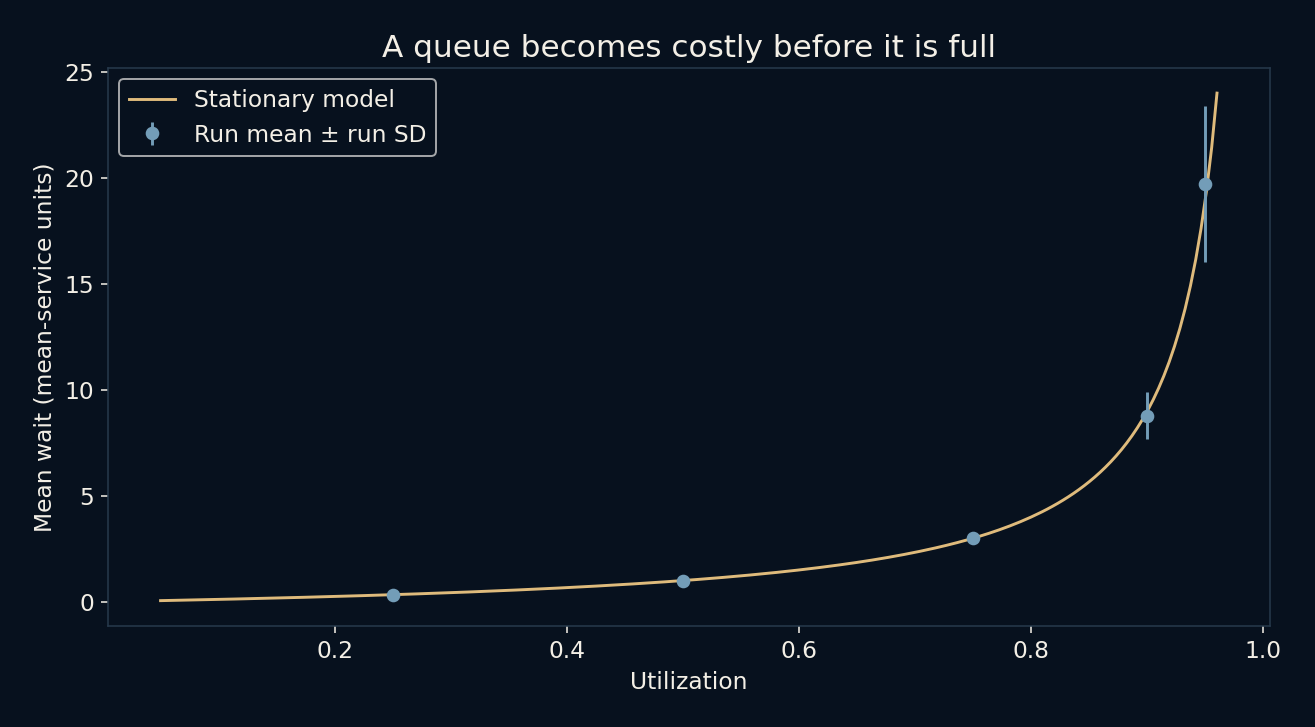
For this ideal stationary model, mean waiting time before service is utilization divided by one minus utilization, measured in mean-service units. At 50% utilization the answer is 1. At 75% it is 3, at 90% it is 9, and at 95% it is 19. This is waiting alone, so the average service time must be added to obtain total time in the system.
The local simulation measured means of 0.996, 3.001, 8.775 and 19.728 at those four loads. They follow the curved relationship without matching it exactly. Increasing utilization from 90% to 95% barely changes the apparent busyness, but the theoretical mean wait more than doubles. The small remaining recovery margin is doing substantial work.
The average hides an uneven experience
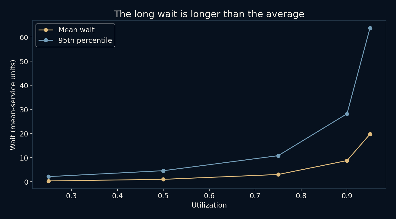
A mean of nineteen service units does not mean every job waits nineteen units. Some arrivals find an empty counter and wait zero. Others land in a long congestion episode. At 95% utilization, the simulated 95th percentile was about 63.734 units. Roughly one in twenty retained waits exceeded that threshold in this pooled simulation.
At 50% utilization, the measured 95th percentile was about 4.579 units, against a mean near one. Percentiles reveal a different part of the experience from an average. They are also estimates from finite data. A rare, unusually long congestion episode can change both the mean and the tail, especially when the load is high.
Starting empty is an advantage
Every simulated counter starts empty. Measuring immediately would give the system a temporary benefit that a long-running queue might not enjoy. The experiment discards the first 10,000 arrivals of each run, then records 50,000 waits. Twelve separate runs at each load expose some variation that one attractive curve could conceal.
Discarding a warmup does not prove the remaining sample is perfectly stationary. At 95% utilization, the standard deviation of the twelve run means was about 3.678 units, much larger than at lighter loads. Successive waits within one queue are dependent because they share a backlog. Treating every wait as an independent observation would exaggerate how much evidence the run contains.
A useful warning, not a staffing calculator
Real services can have several workers, priorities, appointments, batching, breaks or customers who leave. Arrival bursts may be coordinated, and service times may have a very different distribution. Those choices alter the formula and the practical response. These synthetic numbers are not measurements of a website, hospital, shop or call centre.
What travels well is the mechanism: when demand fluctuates, a system needs room to recover after busy spells. Capacity planning should examine the actual workload and the waiting experience that matters, including tail delays. A high utilization figure can look efficient while leaving very little resilience. The right target cannot be chosen from this one model alone.
Further reading
MIT: single-server exponential queue model ↗NumPy: exponential sampling ↗NumPy: quantiles ↗Original documentation and useful background.