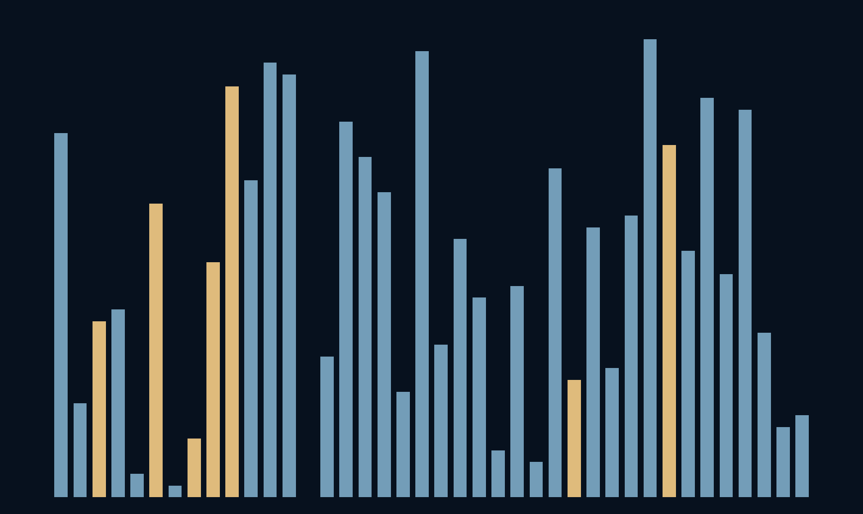
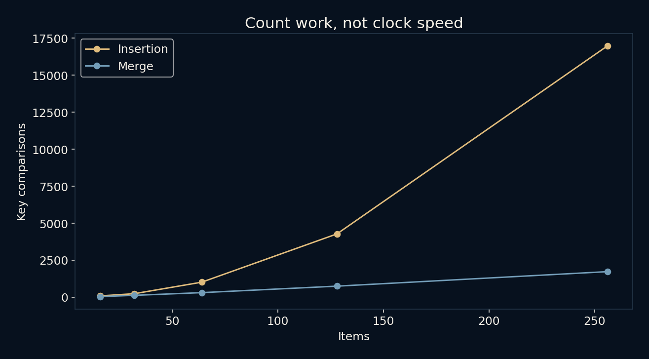
The same 256 numbers needed 16,973 comparisons in one method and 1,728 in another.
Both local programs produced the correct sorted list. Neither used a faster computer than the other. One inserted items into an already ordered prefix; the other split the list, sorted its halves and merged them. The difference is a small, concrete example of algorithm design. We count a specific kind of work rather than claiming a measured speedup.
A good algorithm can remove questions before the machine has to answer them.
Make room inside a sorted hand
Insertion sort resembles arranging a hand of numbered cards. Take the next item, compare it with the items to its left and move larger ones aside until the new item fits. After each insertion, the prefix is sorted. The procedure is straightforward and can do very little work when the incoming order is already helpful.
Our counter increases whenever the implementation compares the inserted key with an existing key. It does not count a loop-bound check as a key comparison. Moving a value, copying a list and allocating memory are also outside this counter. Defining the unit matters: without that definition, two charts labeled “operations” could be measuring quite different things.
Sorted halves make a simpler conversation
Merge sort breaks the list into halves until the pieces are trivial, then joins sorted pieces by comparing their current front items. The smaller front moves to the output, and only that side advances. Once one side is empty, the remainder of the other side can be copied without further key comparisons.
At 256 randomly permuted distinct integers, the tested merge implementation used 1,728 comparisons while insertion used 16,973. At 16 items, the corresponding counts were 42 and 90. These are actual counts for the selected inputs, not formulas predicting every possible list. Both algorithms were checked against the exact ascending integers.
Repeated passes versus repeated levels
In reverse order, insertion sort compares each new key with every earlier key. For n items, the comparison total is n(n−1)/2. At 256 items that is 32,640. Merge sort instead has a sequence of splitting levels, with merging work distributed across the items at each level. This motivates the familiar quadratic versus n-log-n growth descriptions.
Growth notation describes how a cost scales under stated conditions; it is not a stopwatch reading. Constants, data representation and implementation details still matter. The smaller-count algorithm in an educational script is not automatically the best implementation for every tiny list. The important distinction is between making each step faster and needing fewer steps as the problem grows.
An already sorted list tells another story
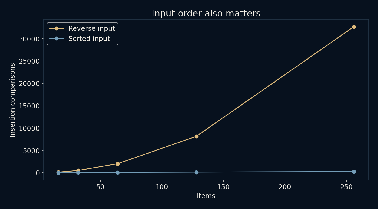
For the same insertion routine, an ascending list of 256 items needs only 255 key comparisons: each new item fits immediately after the previous one. Reverse order needs 32,640. That wide gap comes from the input arrangement, not from changing the algorithm or hardware. A single “sorting cost” number would hide it.
The experiment therefore plots sorted and reverse-ordered cases separately from the seeded permutations. The random examples contain distinct integers and represent only one draw per size. They are useful fixtures for comparing these implementations, but they are not an exhaustive average-case study over every permutation or over duplicate-heavy application data.
A comparison is not the entire bill
Production sorting has to consider memory, moves, expensive comparison functions, stability and partially ordered input. Python’s built-in sorting is an engineered adaptive stable implementation, not either small teaching routine used here. Replacing it with this script would not follow from the comparison chart. We did not time or benchmark the built-in sorter.
What the chart offers is a way to ask a better question before buying more computation. Is the system repeating avoidable work? Can a different organization of the problem reduce that repetition? Measure the real workload afterward, including the costs omitted by the simplified counter. An algorithmic insight becomes useful when its accounting matches the task that actually matters.
Further reading
Princeton Algorithms: elementary sorts ↗Princeton Algorithms: mergesort ↗Python: sorting techniques ↗Original documentation and useful background.