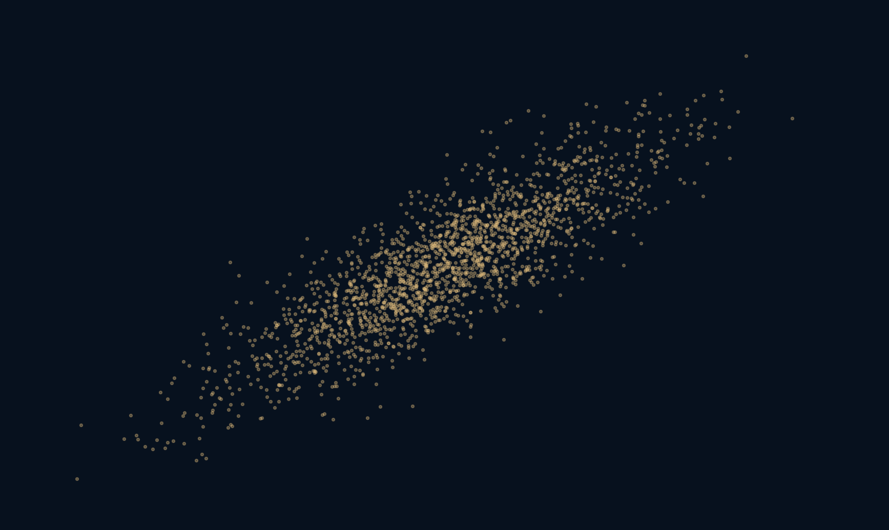
The relationship is real in the data. The story attached to it may not be.
A scatterplot with an unmistakable upward tilt invites a simple explanation: when one thing rises, it makes the other rise. But the picture does not contain that arrow of influence. Both measurements might respond to something else. To make this ambiguity visible, we can build a world where the generating process is known, then hide one ingredient from the first plot. The resulting correlation is strong, even though the construction never uses x to generate y.
A pattern describes what moved together. A causal claim asks what would change if we intervened.
One hidden ingredient enters both measurements
The experiment creates 2,000 rows using seed 941. Each row has a standard normal value z. We construct x as twice z plus one independent standard normal noise value, and y as three times z plus a separate independent noise value. All rows are generated under the same rule. Larger z therefore tends to produce larger values of both x and y.
In this particular construction, neither measurement feeds into the other. Their common ingredient produces the association. We know that because we wrote the generating equations, not because the scatterplot revealed their causal structure. A similar-looking plot from real observations could have several different explanations, including direct influence, reverse influence, shared causes or selection effects.
A strong coefficient is not an explanation
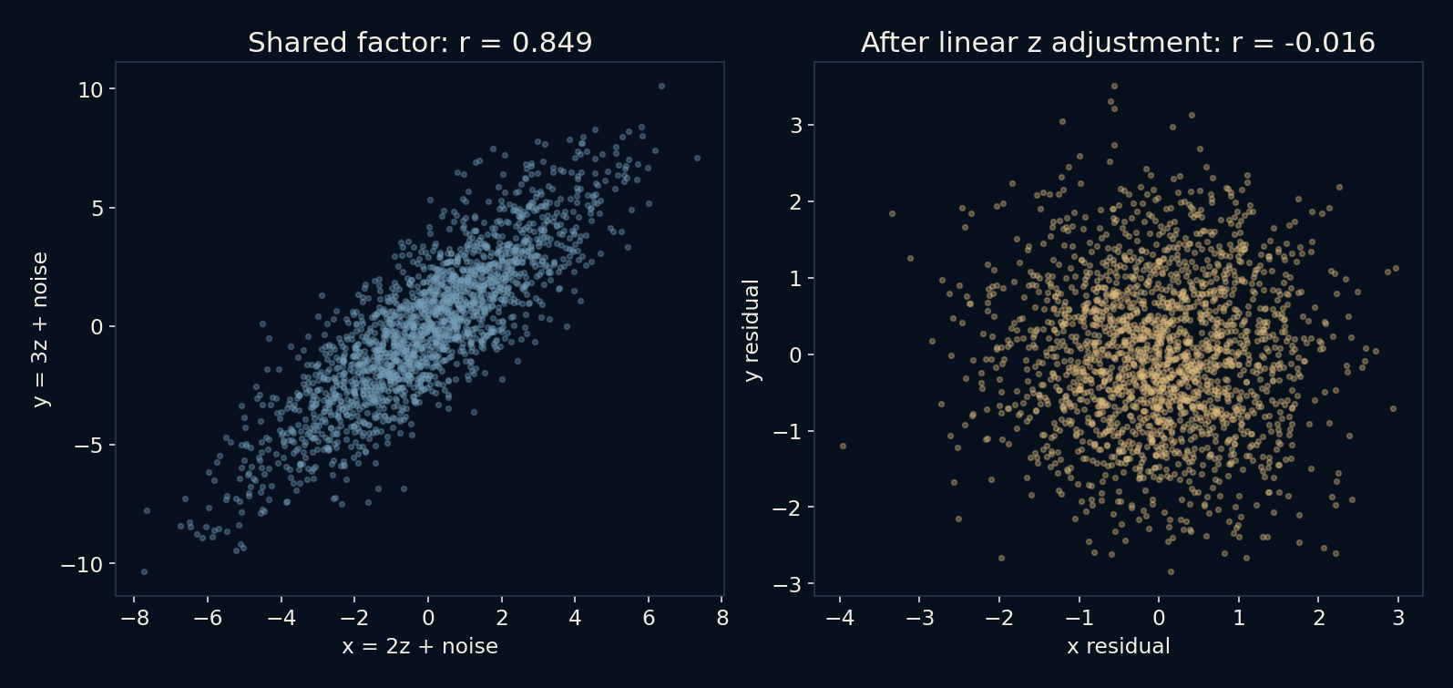
Pearson correlation summarizes linear association after accounting for each variable's scale. Its value lies between minus one and one for nonconstant inputs. Here the raw sample correlation is about 0.8494. That is a strong positive linear pattern in these generated rows. It does not mean an 84.94 percent chance of causation, nor that changing x by one unit would change y by 0.8494 units.
The coefficient is also not a detector of every kind of relationship. A curved pattern can have little linear correlation, and a few unusual points can strongly affect a sample value. Looking at the scatterplot alongside the number helps describe what was measured. Neither view supplies the missing information about which interventions would change which outcomes.
The known generating equations also let us calculate the population coefficient before sampling. Independence makes Var(x) = 2² + 1 = 5, Var(y) = 3² + 1 = 10, and Cov(x, y) = 2 × 3 = 6. Hence the population correlation is 6 divided by the square root of 50, about 0.84853, close to but distinct from the observed 0.84938. The population regression slope of y on x is 6/5, or 1.2, even though changing x alone has zero effect on y in this world. A regression slope and an intervention effect need not be the same number.
Remove the fitted linear part of z
Next, fit a separate straight line for x against z and for y against z, including an intercept in each fit. Subtract each fitted value from its observation. These leftovers are residuals: the parts not explained by the fitted linear relationship with z. Correlating the two residual arrays gives about -0.01591, close to zero in this sample rather than exactly zero.
The large change is consistent with the known construction: the shared linear component has been removed, leaving mostly independent noise. This is an illustration of adjustment in a deliberately favourable setting. It is not a procedure that discovers the right control variable from an unknown dataset, and the small residual correlation alone would not prove the absence of a causal effect in a real study.
The same values tell a different story in different rows
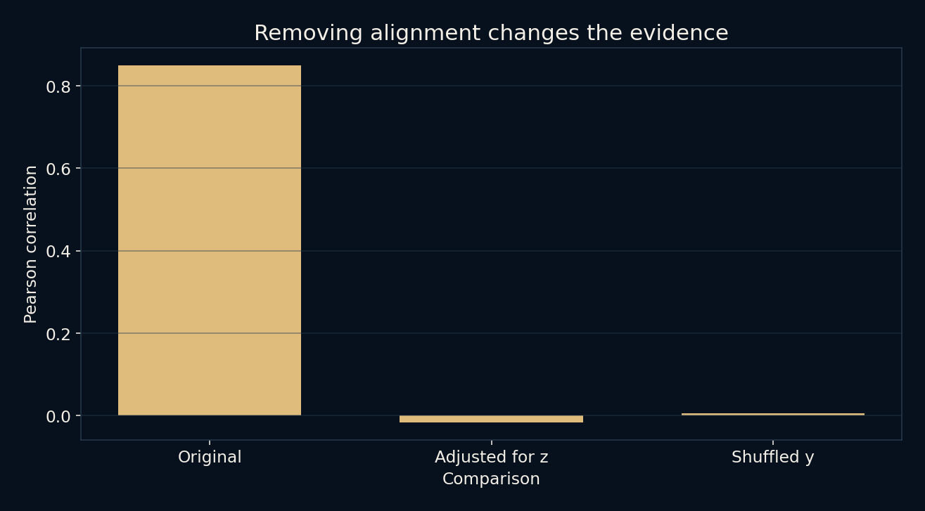
A separate comparison shuffles the original y values while leaving x in place. Every y value remains in the dataset, so its distribution and average stay unchanged. What disappears is the original row correspondence. The resulting correlation is about 0.005705. This makes a simple point: association depends on which values belong together, not just on the two columns considered separately.
The shuffled result is one seeded permutation, not a full permutation test or a significance calculation. More importantly, shuffling is not the same as assigning x at random and observing a new outcome. It changes a recorded pairing, not the process that generated the measurements. Destroying an association in a spreadsheet does not explain the original association in the world.
Controlling for everything is not a causal strategy
Real data do not arrive with trustworthy generating equations attached. A relevant common cause might be unmeasured, measured with error or connected to the outcome nonlinearly. The useful variables to adjust for depend on the causal question and the assumed relationships. Collecting more columns is not the same as identifying those relationships.
Adjustment can also remove part of an effect you meant to measure, for example when controlling for an intermediate consequence. Conditioning on a shared consequence of two variables can create an association instead of removing one. Those possibilities are why the advice to control for all available variables is unsafe. Study design, subject knowledge and explicit assumptions matter before a regression is fitted.
Two worlds can draw the same kind of cloud
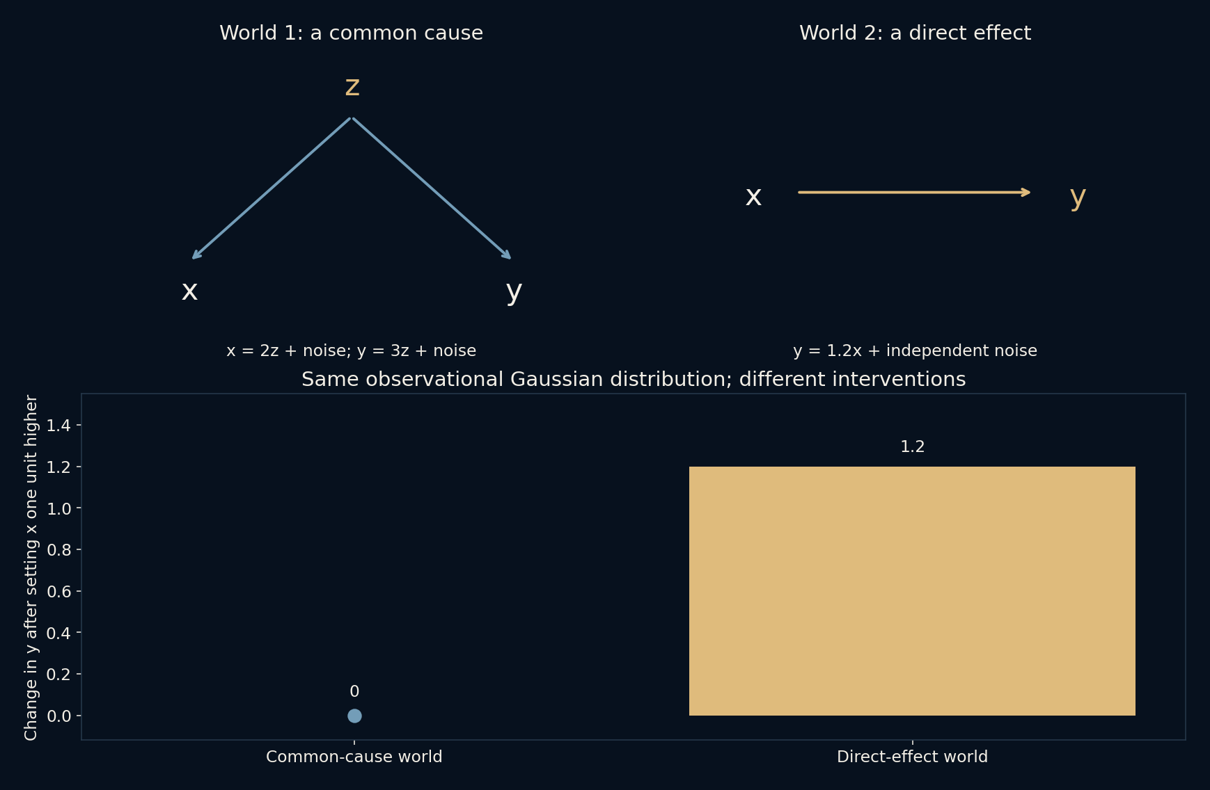
Build a second world in which x is normal with mean zero and variance five, and y equals 1.2x plus independent normal noise of variance 2.8. Here x really is an input to y. Nevertheless, the observable pair has exactly the same joint Gaussian distribution as in the common-cause world: both means are zero, the variances are five and ten, and the covariance is six. Equal means and covariance determine a joint Gaussian distribution. This is equality of distributions, not a claim that two random samples match point for point.
Now intervene within each model, raising x by one while holding its other external ingredients fixed. The common-cause equation for y never reads x, so every y remains unchanged. In the direct-effect world, every y rises by 1.2. The script checks both responses and the two observable covariance matrices. No amount of extra observational data from these same two variables would distinguish the stipulated worlds by their distribution alone. An experiment, additional justified knowledge or a different source of evidence is needed to decide which intervention story applies. That conclusion follows from the models we wrote, not from discovering causality in a scatterplot.
Keep the observation and the explanation separate
When shown a compelling association, first ask what each row represents, how observations were selected and which measurements were paired. Then ask what claim is actually being made. Describing co-movement, predicting another value and estimating the effect of an intervention are different tasks. A useful predictive pattern need not supply a valid answer to the intervention question.
The local checks verify row alignment, residual orthogonality to z and the expected strong-raw, small-residual pattern in this fixture. They check implementation properties and a chosen demonstration, not causal identification. The lesson is not to distrust every correlation. It is to let a correlation do its proper job without asking one coefficient to carry an explanation that the evidence has not established.
Further reading
SciPy: Pearson correlation and its interpretation ↗Hernán and Robins: Causal Inference, What If ↗NumPy: least-squares polynomial fitting ↗Original documentation and useful background.