A random way to estimate a very unrandom number

Pi does not change. Our estimate of it does.

There are much better ways to calculate pi than scattering points on a picture. That is precisely why this makes a good explanation of Monte Carlo estimation: the answer is already known, so the uncertainty is visible. We can watch a random procedure approach a fixed quantity without pretending every extra point is an improvement. The useful lesson is not a new way to collect digits. It is how repeated random samples can measure something, and how stubbornly expensive extra certainty can become.

More samples narrow the uncertainty. They do not make luck disappear from an individual run.

TURN AREA INTO COUNTING

A circle hides a probability inside a square

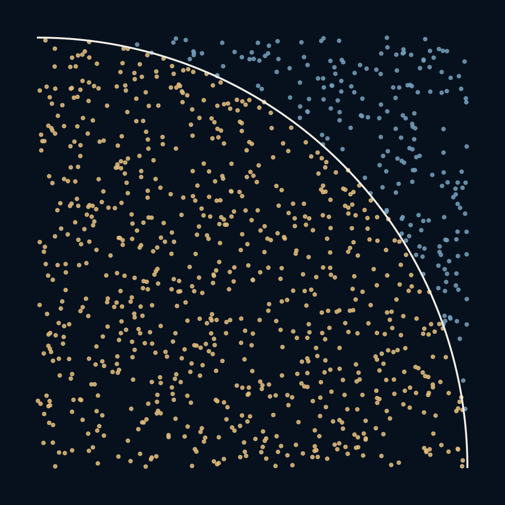
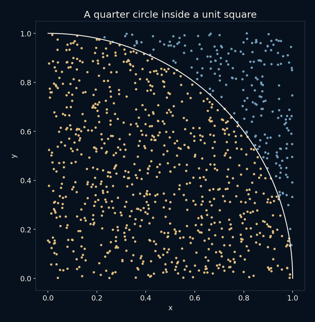
Take the square from zero to one on both axes. A quarter of a unit-radius circle fits inside it. The square's area is one, and the quarter circle's area is pi divided by four. If points are uniformly distributed across the square, the probability of falling inside the curve is therefore pi divided by four. Multiply the observed fraction inside by four and you obtain an estimate of pi.

The membership test is pleasantly small: a point counts as inside when x squared plus y squared is at most one. This replaces an area calculation with a count of yes-or-no outcomes. It also exposes the assumptions. Unevenly placed points would estimate a different probability, and correlated samples would change the uncertainty calculation.

Uniform points fill a unit square, with a white quarter-circle boundary separating mostly gold inner points from blue outer points. — FIG 01A separate 1,000-point illustration uses seed 931. Gold marks x² + y² ≤ 1; blue marks points outside the quarter circle.

ONE RUN

The trace can wander in the right general direction

With only a few points, moving one from outside to inside has a large effect on the fraction. With many points, one point has less influence. That makes longer runs look steadier, but it does not make their errors decrease at every step. A lucky short estimate can be closer than a later, less lucky one. A graph that only shows the smooth-looking part would hide this ordinary behaviour.

A fixed random seed makes the demonstration repeatable. It does not make the particular result inevitable in other runs, and it is not a quality certificate for a random-number generator. Here the seed is a way to keep the illustrations and numbers consistent when the experiment is rerun.

REPEAT THE WHOLE EXPERIMENT

A distribution is more honest than a favourite attempt

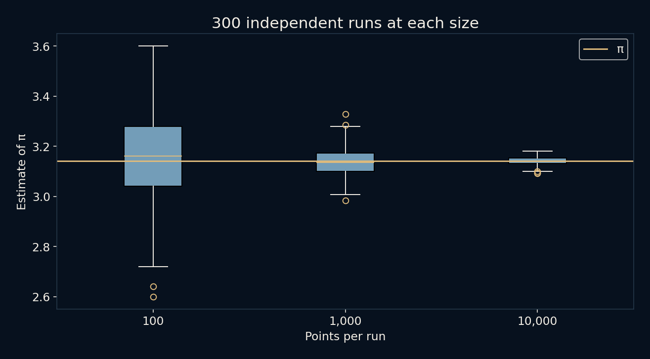
We repeated the estimator 300 times at each of three sample sizes: 100, 1,000 and 10,000 points. The mean estimates were about 3.1477, 3.1378 and 3.1413. Reporting those means alone would make the method look steadier than one run actually is, because each mean combines many separate attempts.

To show the spread, we also measured each estimate's error relative to pi and took the root mean square across the 300 attempts. Those RMS errors were approximately 0.1608, 0.0530 and 0.0158. These are observed summaries of this seeded repeated experiment. They describe a distribution of attempts rather than a guarantee for the next estimate.

Three boxplots for 100, 1,000 and 10,000 points narrow around pi as sample size grows. — FIG 02Each boxplot summarizes 300 runs at its sample size, using seed 930. Boxes show the middle half of estimates; the gold horizontal line is π.

THE PRICE OF PRECISION

Four times the work buys roughly half the typical error

For independent uniform samples, the inside count follows a binomial model. The standard deviation of this estimator decreases in proportion to one divided by the square root of the sample count. Doubling the number of points therefore does not usually halve the uncertainty. Roughly four times as many are needed for that reduction, and a tenfold reduction calls for about a hundred times as many.

The three observed RMS values follow that broad pattern, with finite-run variation. The square-root relationship is about the sampling distribution under the model, not a promise that every displayed curve behaves smoothly. It is also a reason to seek a better estimator instead of simply pouring more computation into an inefficient one.

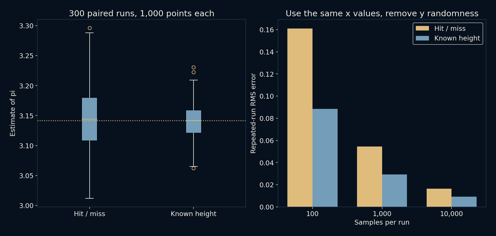
Here the gain also has an analytic explanation. For n independent samples, hit-or-miss variance is (4π − π²)/n, about 2.69677/n. The height estimator’s variance is (32/3 − π²)/n, about 0.79706/n. Its standard deviation is therefore about 0.5437 times as large at the same n. The script independently checks the height’s first and second integrals numerically. This does not make every paired height estimate closer, and the experiment does not measure runtime. It trades access to a known boundary formula for less randomness, an opportunity that another integral may not offer.

WHY USE IT AT ALL

The method earns its keep on harder shapes

For pi, direct numerical methods are far more efficient. Monte Carlo becomes attractive when the quantity is difficult to evaluate directly but random examples are relatively easy to generate. Integration in a complicated space and simulated outcomes are common settings. The same basic pattern appears: define a quantity, draw samples under a stated distribution, and use a summary with an uncertainty estimate.

The distribution matters as much as the sample count. A million samples from the wrong model can give a very precise answer to the wrong question. Real simulations also need checks on the assumptions, numerical implementation and dependence between samples. The square-and-circle picture avoids most of those complications so that the statistical idea can be seen clearly.

REMOVE A LAYER OF CHANCE

Use what you know before drawing more points

For any fixed x in the unit square, the height of the quarter circle is the square root of 1 minus x squared. A uniform y lands below that height with exactly that probability. Instead of drawing y and recording a noisy zero or one, we can average the known height itself and multiply by four. Both estimators target pi, but the second has already averaged over the vertical randomness. This is a concrete example of using conditional information to reduce variance.

The new comparison uses seed 1930 and 300 paired runs at each original sample size. Each pair uses the same x coordinates. At 1,000 samples, the hit-or-miss RMS error is 0.05439, while the height estimator gives 0.02928. At 100 samples the values are 0.16114 and 0.08845; at 10,000 they are 0.01643 and 0.00916. These are a separate experiment from the earlier seed-930 results. The paired setup makes the comparison interpretable without selecting a particularly lucky run from either method.

The known-height estimator has narrower repeated-run spread and lower RMS error than hit-or-miss in the tested samples. — FIG 03Seed 1930, 300 paired runs per size. Each pair shares its x values. Boxplots show the 1,000-sample runs; bars show empirical RMS at all three sizes, not guaranteed errors.

READ THE RESULT

Ask for the spread, not just the impressive decimal

When a simulation prints many decimal places, it is easy to mistake formatting for knowledge. A result such as 3.141309 is a computed value, but its digits do not all carry equal certainty. The repeated-run spread tells us much more about the procedure than the number of characters the program chose to print.

Our checks verify the membership boundary on known points, keep every estimate between zero and four, and confirm the observed RMS ordering for these sample sizes. They do not establish universal monotonic improvement. The circle gives us a known answer with which to practise being sceptical of a simulation, before the answer is no longer available for comparison.