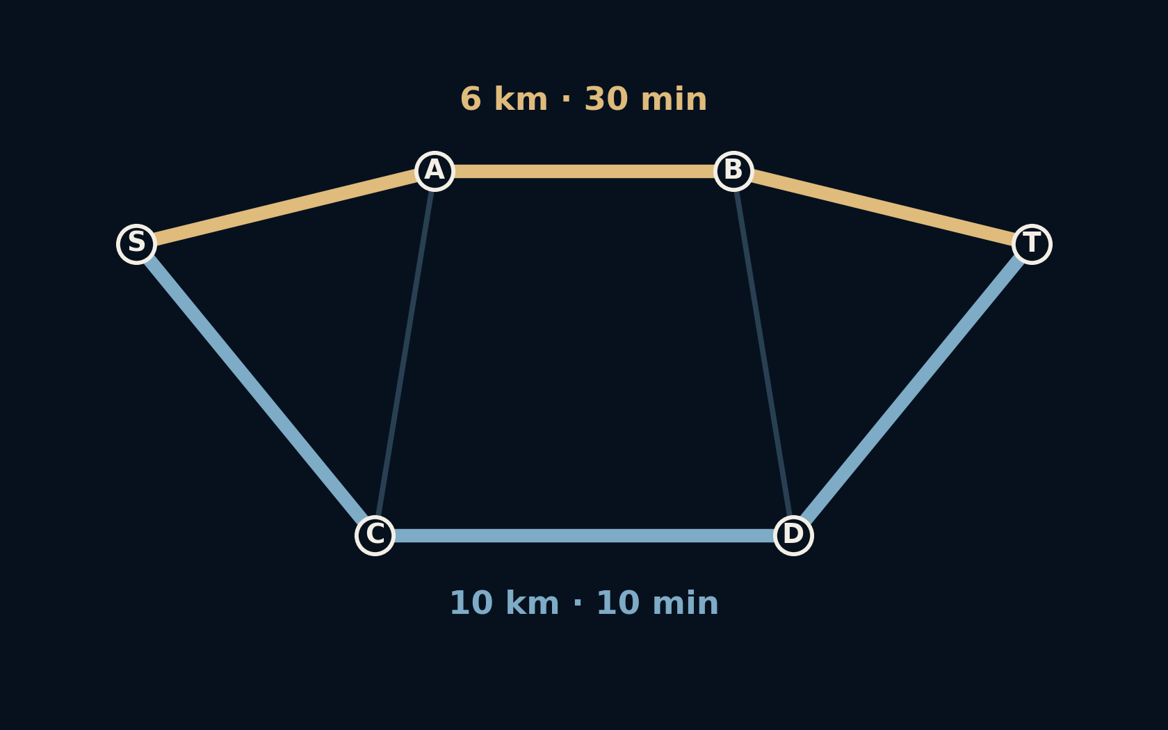
The route is four kilometres longer. It arrives twenty minutes earlier.
That sounds like a navigation mistake until the map acquires a second set of numbers. Distance describes how much road you cover. Time also depends on how quickly you can cover it. In this small, deliberately invented network, asking for one rather than the other changes the answer completely.
A route is only best after you decide what “best” costs.
Two perfectly reasonable answers
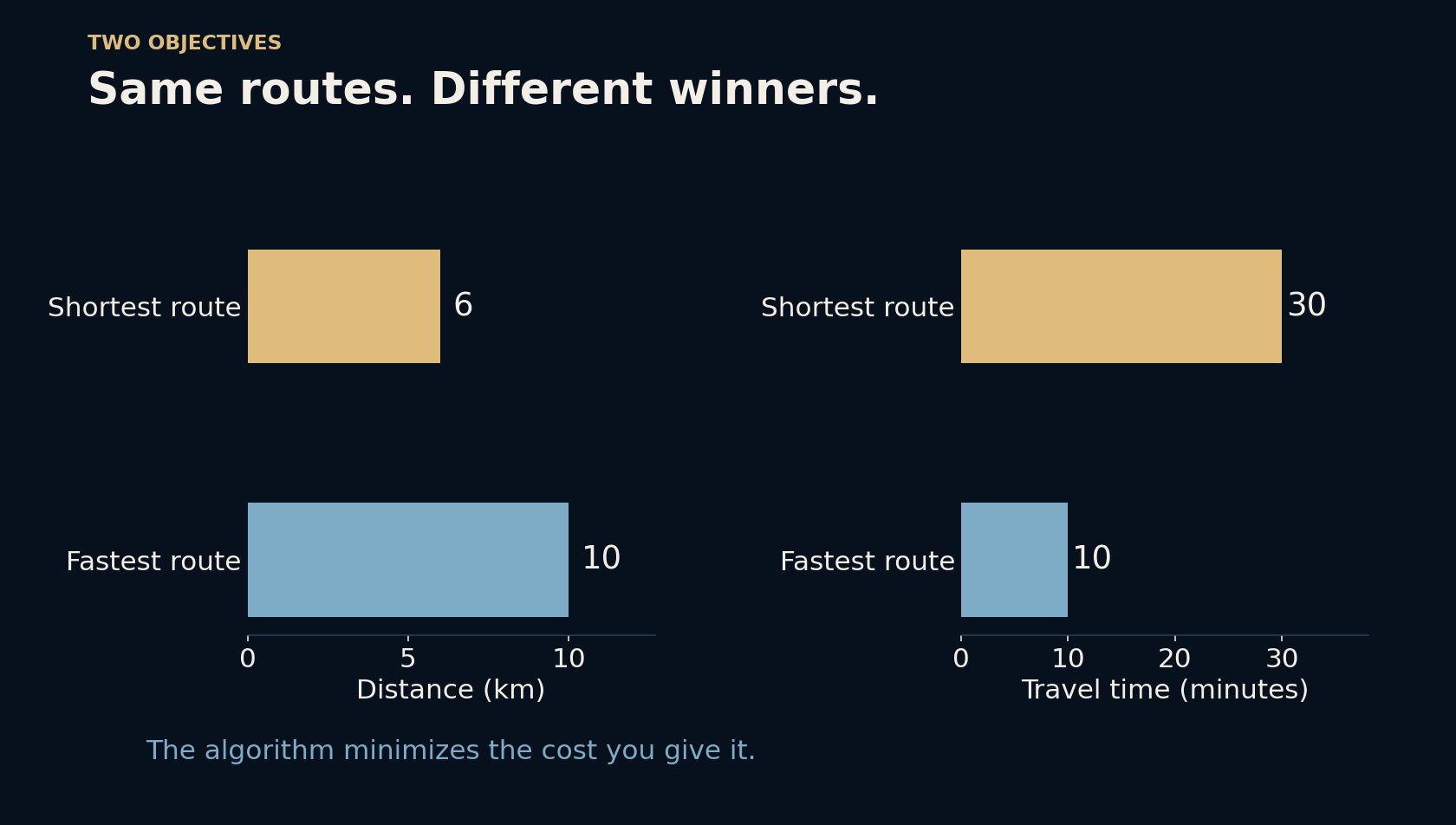
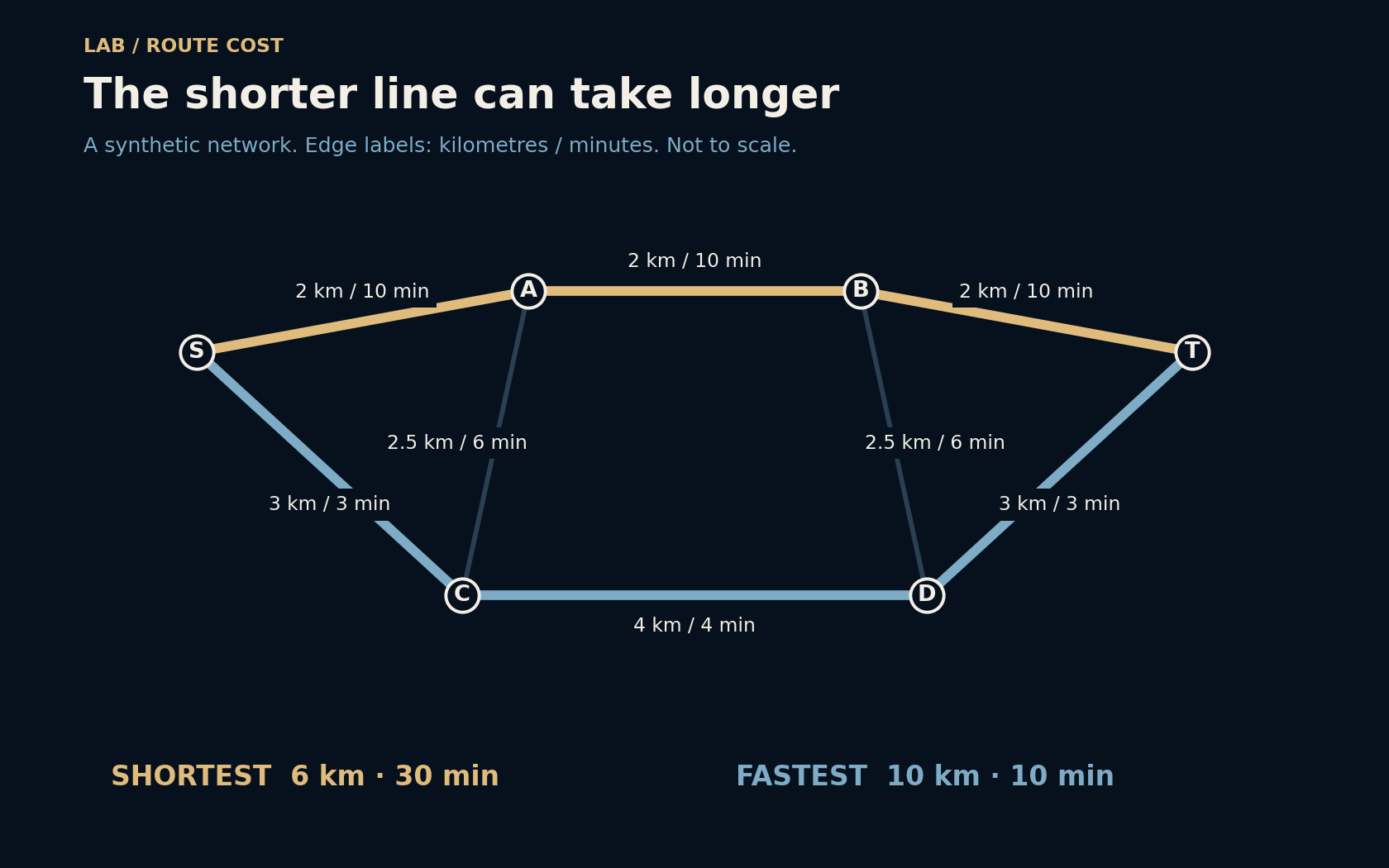
Start at S and finish at T. The upper road passes A and B: three two-kilometre segments, six kilometres altogether. Each segment has an assumed speed of 12 km/h, so each takes ten minutes. The lower road passes C and D. Its segments total ten kilometres, but the assumed speed is 60 km/h throughout. That journey takes ten minutes altogether.
The distance winner therefore needs thirty minutes, while the time winner needs ten. Neither answer contradicts the other. They solve different questions. The little connecting roads make this a network rather than a choice between two isolated lines, and they will matter when one of our assumptions changes.
A map becomes a list of costs
To a graph algorithm, a junction is a node and a usable connection is an edge. Each edge gets a weight: the cost of using it. For the first calculation, the weight is kilometres. For the second, it is minutes, computed as distance divided by speed, then multiplied by sixty. The geometry of the drawing never enters the calculation.
That last detail is easy to miss. A neatly drawn line is not evidence of a short journey. Our diagram is not to scale, and its distances are assigned explicitly. Likewise, a real routing system needs usable road connections and restrictions, not just straight-line measurements between places. A bridge that looks nearby may be inaccessible from your side of the river.
Dijkstra follows the cheapest known frontier
Dijkstra’s algorithm starts with cost zero at S and an unknown cost everywhere else. It repeatedly takes the unsettled node with the lowest known total, checks its outgoing connections, and improves a neighbour’s total when it finds a cheaper way there. It also remembers which preceding node supplied that improvement, so the winning path can be reconstructed.
The requirement that edge weights are nonnegative makes this strategy work: continuing along a path cannot undo a cost already paid. Once the destination is settled, its cost is minimal under these assumptions. The algorithm does not understand lateness, scenic roads, or convenience. Those priorities enter through the model and its weights, before the search begins.
Eighteen minutes changes the picture
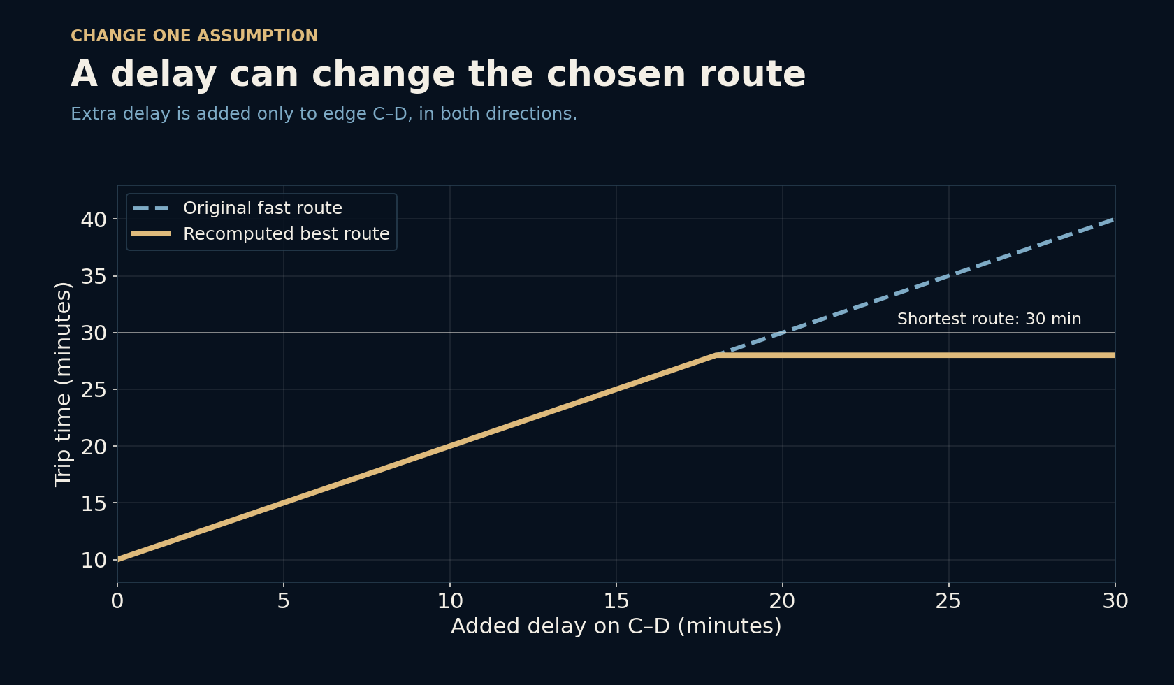
Now add a delay to the C–D connection and recalculate. The original fast route takes ten minutes plus the delay. At an eighteen-minute delay, it ties with a different route at twenty-eight minutes. With a larger delay, the optimum can avoid that connection by using the cross-links: S–C–A–B–D–T. Its distance is thirteen kilometres.
This is why an old winning route need not remain the winner. At a twenty-minute delay, simply keeping the original fast route produces thirty minutes; searching again finds twenty-eight. The result is still only as good as the updated assumptions. Here the delay is a fixed surcharge in both directions, not a traffic forecast that changes while someone travels.
A single number hides your priorities
A person may prefer fewer transfers, avoid tolls, need a step-free route, or accept a slower road that feels safer. Some requirements should remove unusable edges before searching. Others can become costs or separate choices shown to the traveller. Folding everything into one score is possible, but the conversion is a decision: how many extra minutes is one toll worth?
Even “fastest” needs a definition. The lowest expected travel time can differ from the route most likely to meet a deadline. Our fixed-speed example contains no uncertainty, so it cannot settle that question. It explains one clean distinction without pretending that the whole task of navigation is a handful of additions.
Read the objective before trusting the answer
When two route suggestions disagree, compare what each is minimizing and which restrictions it knows about. Check the departure time, travel mode, closures, and whether the estimate includes walking or waiting. These details can matter more than the apparent directness of the line on the screen.
The same habit travels beyond maps. A delivery plan, a network connection, or a sequence of production steps can all be represented as routes through choices. The search may be exact while the chosen objective is incomplete. Before improving the algorithm, it is often worth asking whether its cost measures the thing that actually matters.
Further reading
NetworkX: Dijkstra path and edge weights ↗SciPy: Dijkstra shortest paths and limitations ↗Original documentation and useful background.