The picture that survives a close look

A circle can be a short instruction

The source shape has centre zero and radius 0.72 in a square spanning minus one to one on each axis. Its inside is defined by the sum of squared coordinates being no greater than the squared radius. That rule can answer whether any chosen point belongs to the circle without storing a colour for every possible position.

This is the useful idea behind vector graphics: represent shapes through geometry and drawing instructions. Paths, fills, strokes and transformations can remain editable as descriptions. A more complex illustration may need many such instructions, but enlarging the coordinate system need not change the underlying shape into a pre-existing grid of larger squares.

Rasterization chooses a finite set of questions

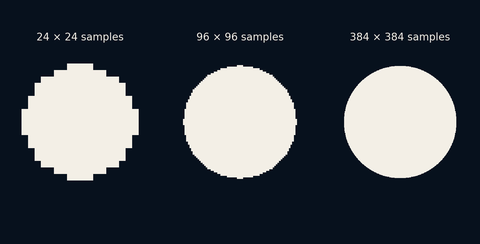
Our rasterizer samples the centre of every pixel and asks whether it is inside the circle. It does this on grids of 24, 96 and 384 samples per side. Each pixel becomes either zero or one. This deliberately simple point test makes the sampling visible; it is not the coverage-antialiased rendering used by many drawing systems.

The circle equation is unchanged between the three images. What changes is the density of questions asked of it. A finer grid follows the curved boundary with smaller steps, while a coarse grid must make broad decisions. The shape did not acquire more mathematical detail; the raster representation acquired more samples of the same geometry.

A small translation reveals another consequence of the centre test. Move the circle by half a coarse-pixel spacing along both axes, about 0.041667 coordinate units each. Its actual area has not changed, but the 24-by-24 binary estimate changes from about 1.66667 to 1.67361. Different centres have crossed the boundary. This is a sampling effect, not evidence that the geometric object grew when it moved or that its source description was damaged.

Enlarging pixels does not ask the shape again

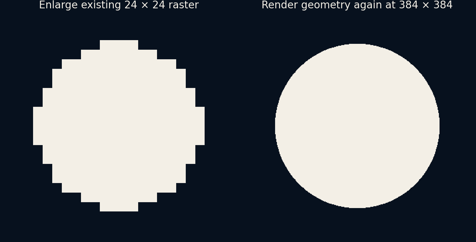
The side-by-side comparison contrasts a 24 by 24 raster enlarged with nearest-neighbour display against a fresh 384 by 384 rendering of the original circle. In the first, each old sample becomes a visible block. In the second, new sample positions are evaluated using the geometric definition.

Other interpolation filters can smooth the enlarged raster and make its blocks less obvious. They estimate intermediate values from the samples available, rather than consulting an original curve that the raster file may no longer contain. That distinction remains even when an enlargement looks attractive. A plausible edge is not automatically a recovered measurement of the original boundary.

This also explains why a smooth-looking export deserves a source check. A filter can soften a jagged outline while leaving the available shape information unchanged. If the intended task is to change the circle's radius or edit a curve, a softened raster still lacks the original editable equation. Appearance at one display size and the ability to make a reliable future edit are different qualities worth checking before discarding the source.

The area gives a second way to compare

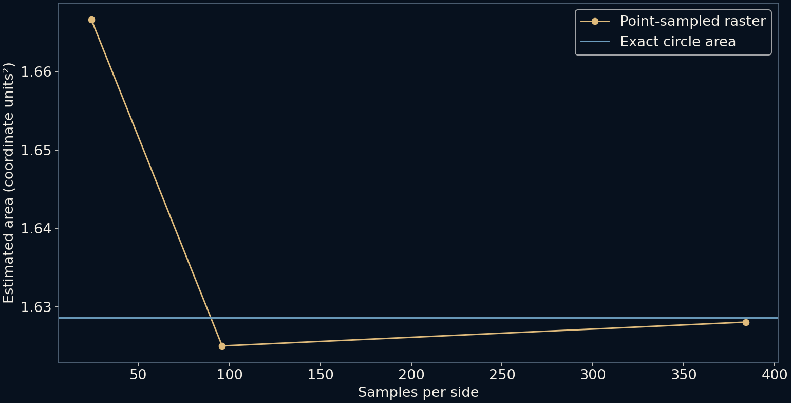
Counting inside pixels and multiplying by pixel area estimates the circle’s area. The exact geometric value is pi times 0.72 squared, about 1.62860 square coordinate units. Our three grids estimate approximately 1.66667, 1.62500 and 1.62804. The finest result is close, but the middle estimate falls below the exact value while the coarsest is above it.

These values explain why resolution alone is not a promise of monotonic accuracy at every step. Boundary alignment with the sample grid matters. For this sequence, absolute error decreases, but a different sequence of resolutions can oscillate. Analytic coverage or more careful integration can answer a different, more accurate area question than a centre-only test.

Every display still ends in pixels

A vector image eventually has to be rasterized for a conventional screen. It does not bypass the pixel grid or guarantee perfect small-size legibility. Thin strokes can vanish, nearby features can merge and filters can alter edges. The advantage is retaining a description from which an appropriate raster can be generated for the required output.

A file format also does not settle the issue by itself. An SVG can embed a raster photograph, and some effects depend on raster processing. Calling a document vector does not make every element resolution-independent. Inspect the actual source objects and export settings when a logo or diagram behaves unexpectedly after scaling.

Antialiasing does not abolish this final grid. It can encode how much of a pixel is covered instead of forcing every boundary pixel fully inside or outside. The resulting intermediate values are useful information, but they do not create room for arbitrarily many separate details inside one displayed pixel. Tiny features can still merge. Coverage also is not a calibrated brightness measurement; the new illustration uses a colour scale to reveal fractional coverage, without testing display gamma or compositing software.

Keep the representation that suits the work

For geometric logos, icons and diagrams, keeping an editable vector source is often useful. For a photograph, a sampled image is a natural record of the capture, and forcing it into a few curves may discard the very texture that matters. Hybrid documents can sensibly use both kinds of representation.

The practical habit is to keep the richest relevant source and generate the final output for its destination. If the source is a fixed raster, choose enough pixels for the intended use and understand what enlargement can only estimate. If the source is geometry, rerender it instead of repeatedly scaling a small exported copy.

Ask more questions within each pixel

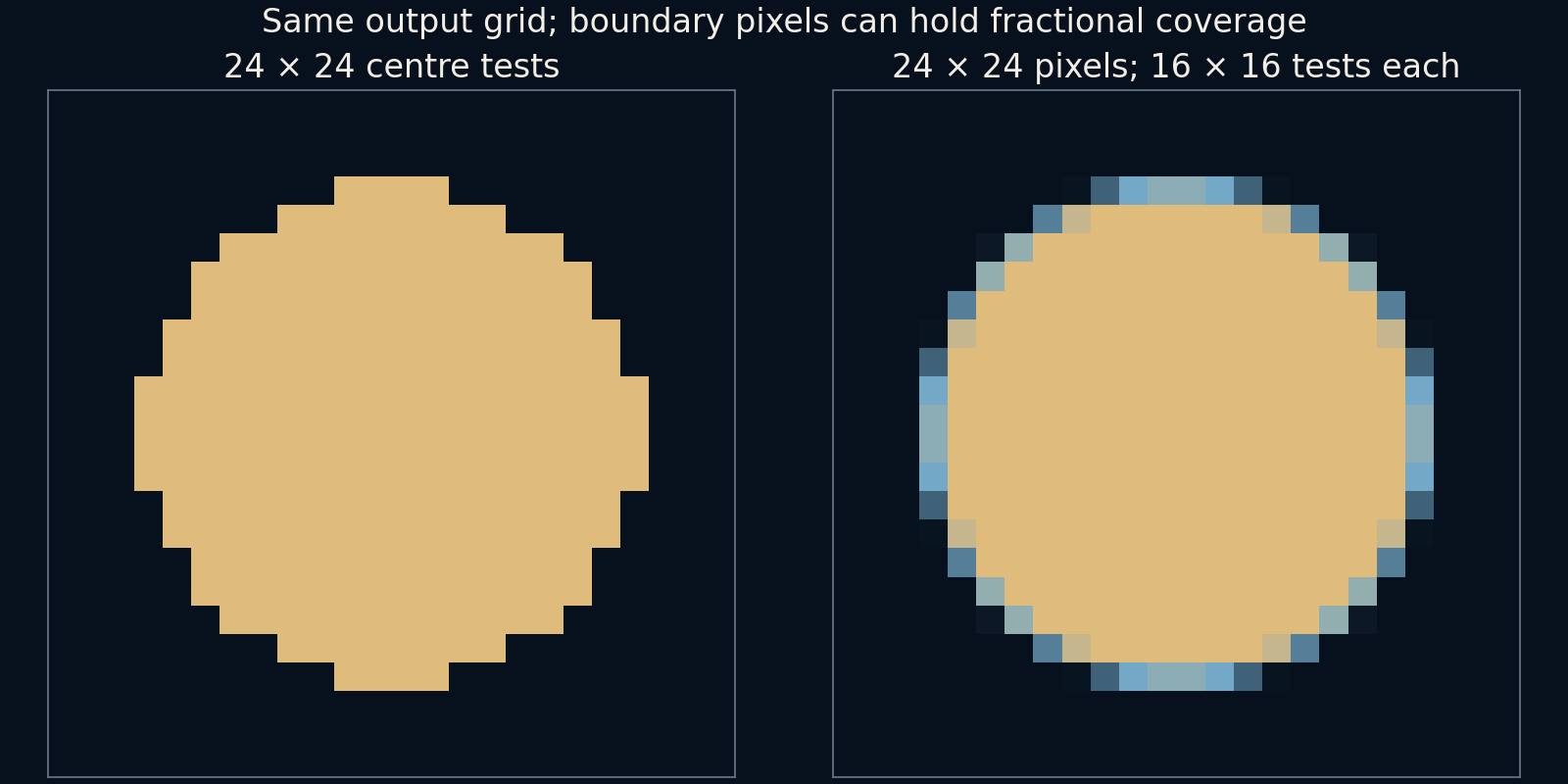
Keep the output at 24 by 24 pixels, but place a regular 16-by-16 array of sample centres inside every pixel. The fraction falling inside the circle estimates that pixel's coverage. We still store only 576 output values, while evaluating the geometry 147,456 times. In this fixture, 60 edge pixels have values strictly between zero and one. The comparison keeps the displayed pixel scale identical so those intermediate boundary values, rather than a larger output, explain the difference.

Summing those coverages times pixel area gives approximately 1.628038 square coordinate units, compared with the exact 1.628602. Here the subpixel sample locations are exactly the same locations as the earlier 384-by-384 grid. Grouping them changes the output representation, not the total sampled area. This finite supersampling is still an estimate, not an analytic integration of the circle's curved boundary. It improves this case without establishing a universal error guarantee for all shapes.

The distinction suggests a practical export check. Inspect the actual destination size, including thin lines, small holes and text, rather than judging only a large preview. Keep geometry for future re-rendering and choose a rasterization method suitable for the smallest features that need to survive. More samples can improve coverage estimates, but no sampling method can preserve every feature at every size. A deliberately simplified small icon can sometimes communicate more clearly than a detailed source merely reduced.