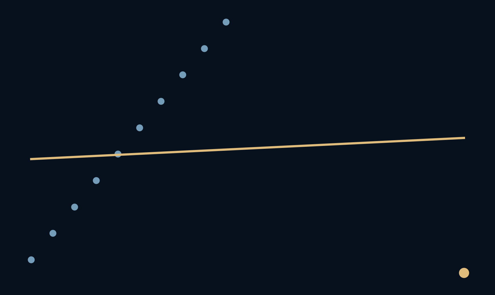
Ten points follow a perfect rising line. Add one point, and the fitted slope nearly vanishes.
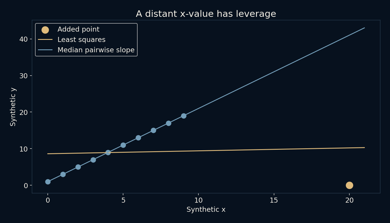
The starting dataset is deliberately plain: x runs from zero to nine and y equals twice x plus one. Every point lies exactly on the same line. Then the experiment adds the point (20, 0). Nothing about the original ten observations changes, yet an ordinary least-squares fit becomes almost flat. The added point has leverage because of where it sits, as well as how far it disagrees.
A fitted line can be balanced around a very unusual point.
What least squares tries to minimize
Ordinary least squares chooses a slope and intercept that minimize the sum of squared vertical residuals. A residual is the observed y value minus the line’s prediction at the same x. Squaring makes negative and positive differences contribute positively, and it makes large differences especially costly. The method is solving a precise optimization problem.
Before the extra point arrives, the best slope is 2 and the intercept is 1, with zero residuals. After adding (20, 0), the fitted slope becomes about 0.08006 and the intercept 8.61782. The new line compromises across all eleven observations. It is not malfunctioning or selectively forgetting the original data.
Distance along x changes the negotiation
The added observation sits far beyond the original x range of zero through nine. Tilting the fitted line changes its predicted value there substantially. This geometric influence is called leverage. A point can have high leverage without being problematic if it lies along the existing trend; the conflict in this fixture comes from its unusually low y value too.
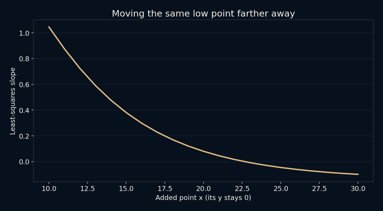
To isolate position, the script holds the added y at zero and moves its x from ten to thirty. The resulting least-squares slopes change as the point moves. This is a controlled sensitivity exercise, not a survey of real outliers. It shows why judging a point only by its vertical distance from the centre of a scatterplot misses part of its influence.
Let many pairs vote on the slope
The comparison fit computes the slope connecting every pair with different x values, then takes the median of those slopes. It sets the intercept to the median of y minus slope times x. In this constructed dataset, 45 pairs among the original ten points all have slope 2. Only ten pairs involve the added point.
The median pairwise slope therefore remains 2, and the median-residual intercept remains 1. This is a transparent resistant construction related to Theil–Sen estimation, with its intercept convention stated explicitly. Its success here comes from the deliberate geometry of the fixture. It is not evidence that one estimator will recover the truth in every noisy or multi-cluster dataset.
A robust fit cannot decide what happened
The gold point could represent a unit error, a different operating regime, a rare valid case or an important failure of the straight-line model. In a real investigation, those possibilities would require context. An algorithm that discounts its influence cannot tell us which explanation is right. An unusual observation may be the most valuable part of the study.
The useful response is to inspect the raw point, check its provenance and compare fits with clearly stated assumptions. Reporting both the sensitivity and the original observation is often more honest than quietly deleting it. If the data contain distinct groups or a curved relationship, a more appropriate model may matter more than a tougher straight-line estimator.
A line is also an extrapolation choice
The original points support a relation only over their observed x range. Extending the blue line to x=20 predicts 41, but that extension is a model assumption rather than a measurement. Our invented new point was designed to disagree with it. Real extrapolation deserves the same separation between what was observed and what a line projects.
A scatterplot, residual check and sensitivity comparison make this separation visible. The aim is not to crown the line that looks most reassuring. It is to understand what controls the conclusion and whether the model matches the question. A tiny change to the dataset can be a large change to the evidence a fitting rule chooses to emphasize.
Further reading
NIST: least-squares fitting ↗SciPy: Theil–Sen slopes and intercept conventions ↗NumPy: polynomial least squares ↗Original documentation and useful background.