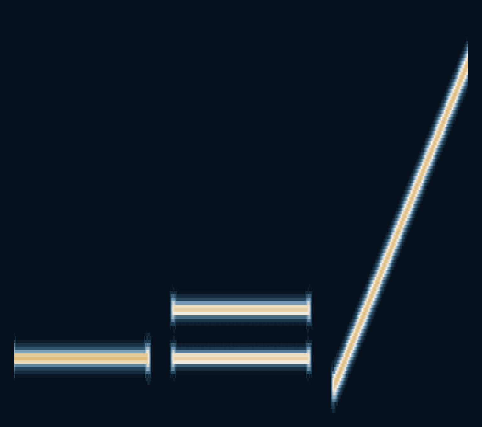
If two notes arrive at once, why does a microphone draw only one line?
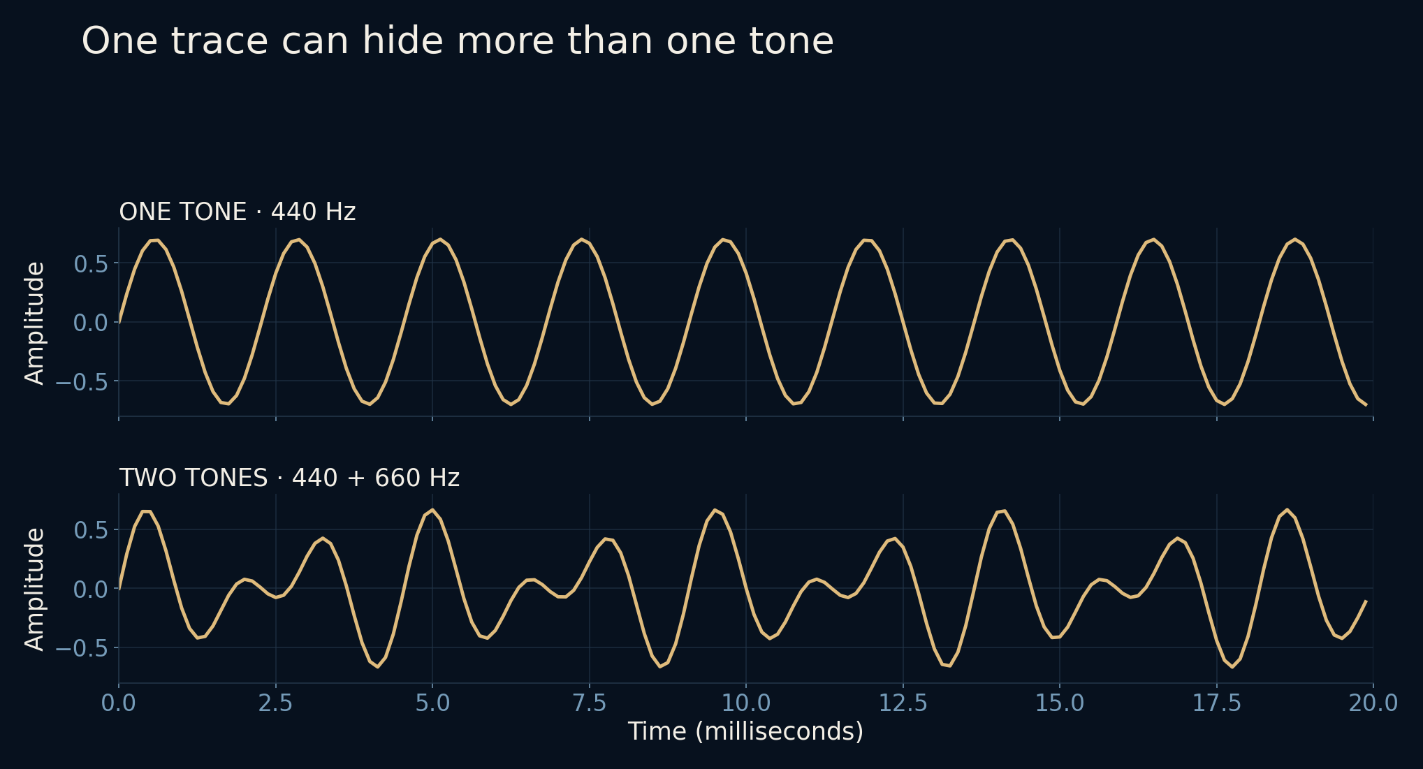
A sound recording is a sequence of pressure measurements, represented as numbers. At each instant, the contributions of different sounds are added together. The familiar waveform follows that sum. It does not give every note a separate lane. To see the ingredients changing over time, we need a different view.
A spectrogram makes time visible without asking it to stand still.
The waveform contains a mixture
Start with a steady 440 Hz sine wave: 440 cycles each second. Its trace rises and falls regularly. Add a 660 Hz sine wave and the shape becomes more complicated. The two contributions have not disappeared; they share the same sequence of values. A Fourier transform describes that sequence in terms of repeating components.
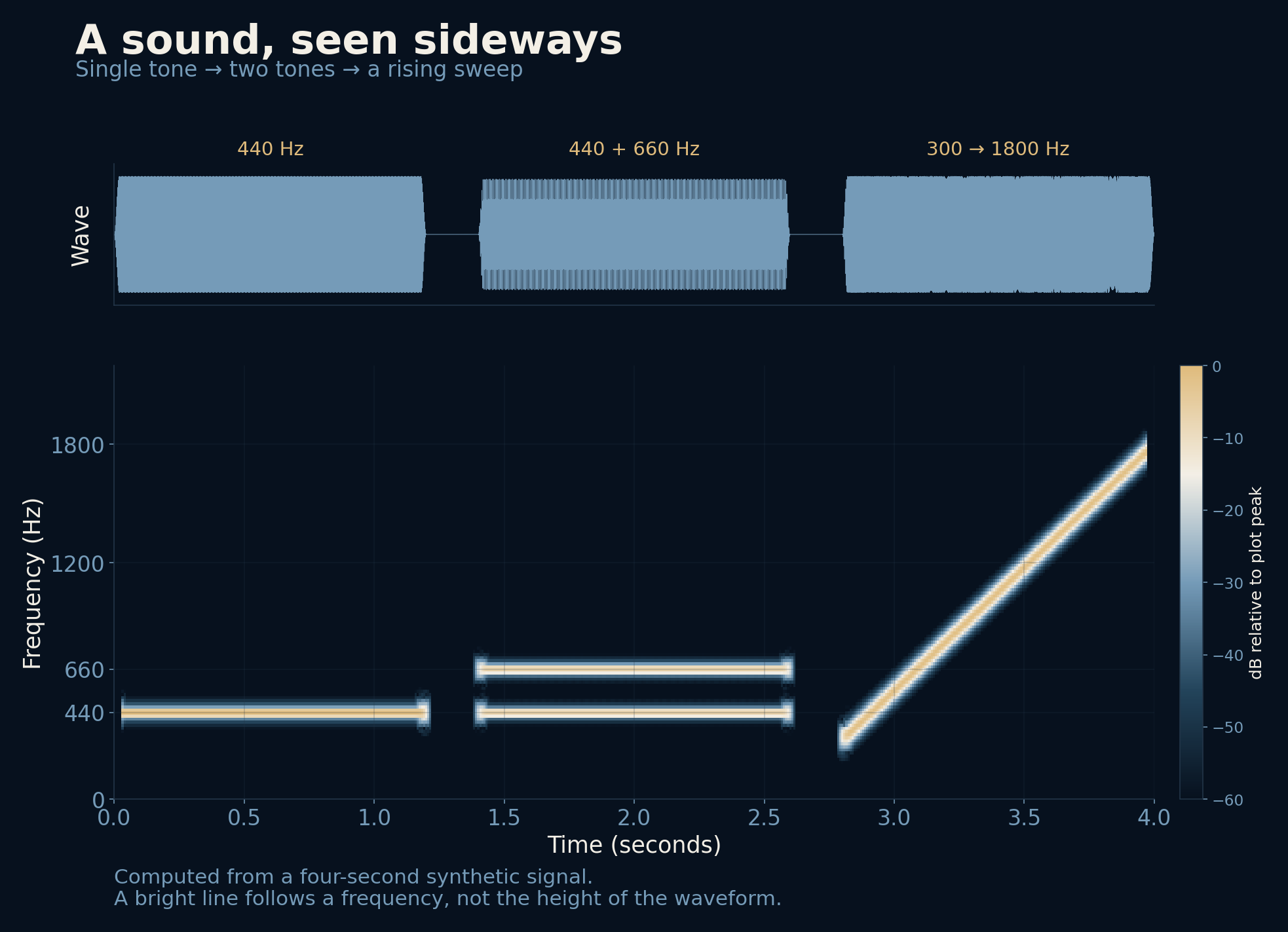
For this article, both tones are generated directly from formulas. The four-second signal begins with 440 Hz, moves to 440 and 660 Hz together, then finishes with a sweep rising from 300 toward 1,800 Hz. Short silent gaps separate the sections. No microphone, song or private recording is involved.
Listen with a moving window
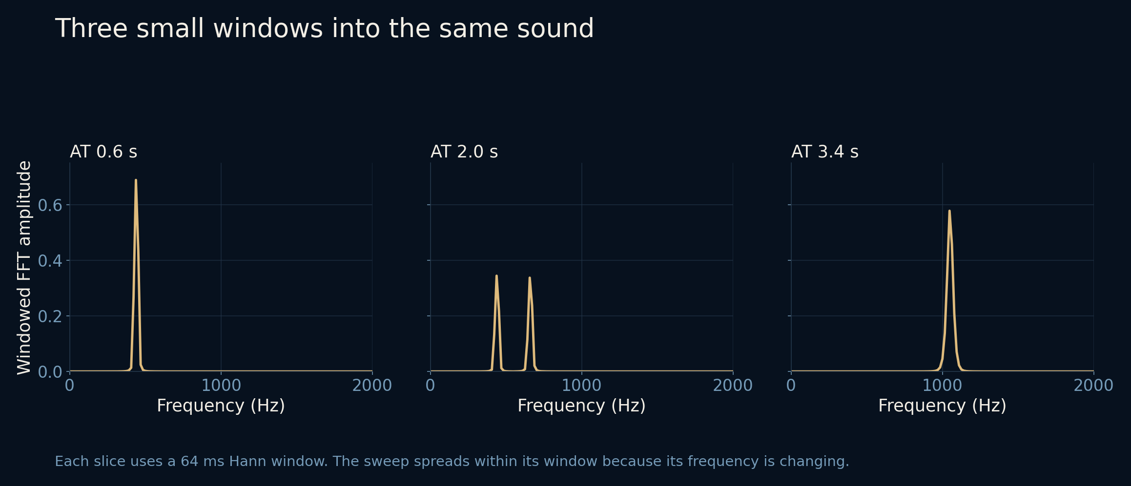
A Fourier transform of the whole recording would tell us which frequencies contributed across the whole interval. It would not keep a convenient timeline of when each appeared. Instead, we take a short piece, analyze it, move forward a little, and repeat. This is the short-time Fourier transform, or STFT.
Before transforming each piece, we taper its edges with a Hann window. Cutting out a segment abruptly can spread its energy across frequencies; the taper reduces that effect, at the cost of broadening spectral peaks. Arrange the resulting spectra as neighboring columns, and their changing strengths become a spectrogram.
Height is frequency, not loudness
Read the main image from left to right. Time travels horizontally. Higher frequencies sit higher on the page, while brighter colors mark stronger components. The first section draws one horizontal stripe. The second draws two. The final sweep climbs diagonally because its frequency is increasing, not because its volume is rising.
The main calculation uses 512 samples per window at 8,000 samples a second: 64 milliseconds of signal. Each window starts 8 milliseconds after the previous one. Its native frequency bins are 15.625 Hz apart. The 440 Hz tone peaks at 437.5 Hz; the 660 Hz tone peaks at 656.25 Hz. Those nearby bin centers are expected, not evidence that the source notes changed.
A longer glance hears a finer difference
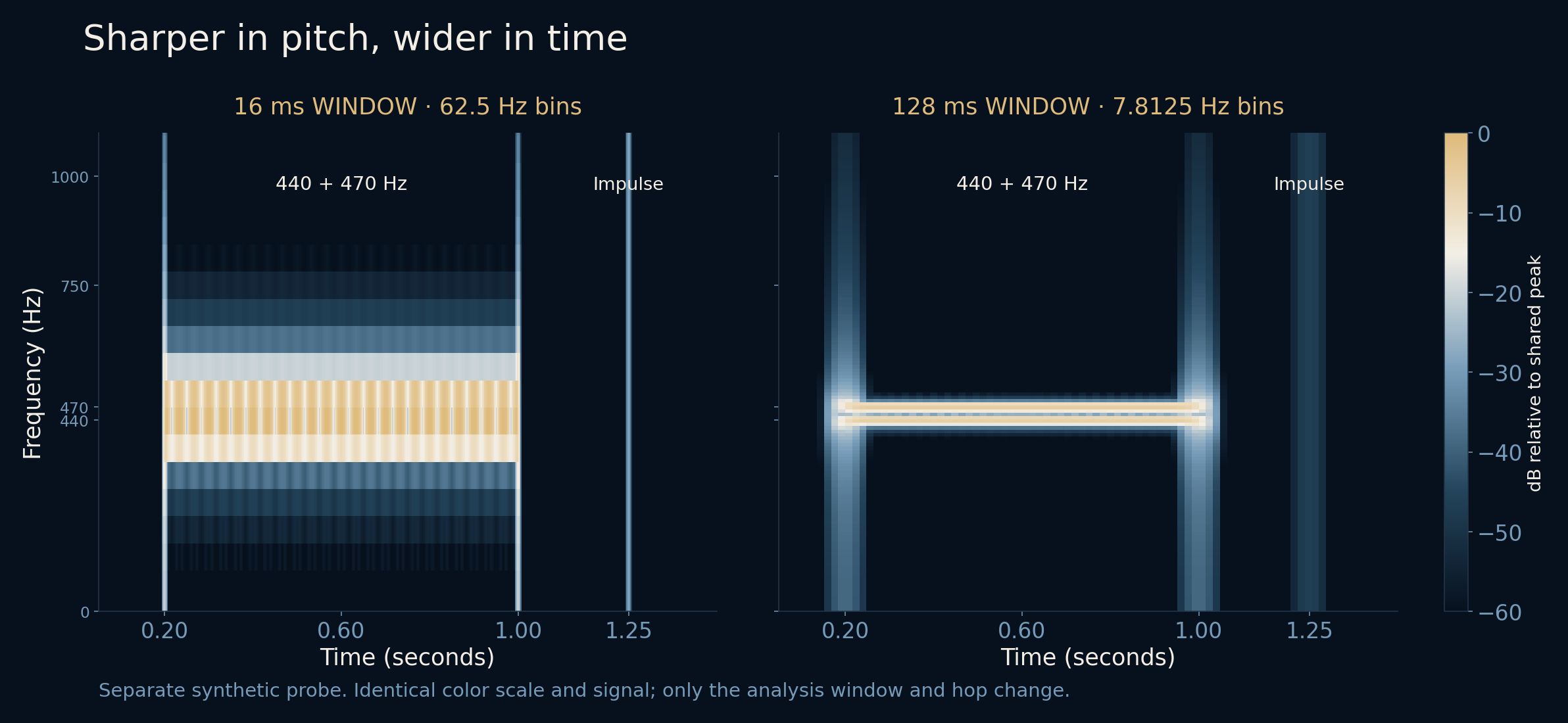
A separate test places 440 and 470 Hz tones together, followed later by a single-sample impulse. With a 16 ms window, the neighboring tones merge into one detected peak. With a 128 ms window, they produce two detected peaks near 437.5 and 468.75 Hz. The longer observation has more evidence for distinguishing their rates.
But look at the impulse. Its mark spreads across more time in the longer-window image. Any analysis window containing that instant can register it. Long windows favor frequency separation; short windows localize sudden changes more tightly. There is no one window that is best for every question.
The colors are choices, too
Our images show decibels relative to a plot peak, with the displayed range running from −60 to 0 dB. They are computed from the windowed transform magnitude. They do not report a sound-level meter reading, and 0 dB here does not mean silence. Changing the reference or color range would change the picture without changing the signal.
Likewise, more overlapping windows make the time axis more densely sampled but do not erase the window-length compromise. Adding zero padding can draw more closely spaced frequency bins without giving the original observation more resolving power. Smooth-looking graphics and genuinely distinguishable tones are different things.
A map is useful because it leaves things out
Once the axes make sense, the picture becomes a useful guide. A stable tone tends to leave a horizontal trace. A frequency sweep bends or slopes. A brief click can spread vertically because it contains a broad range of frequencies. Real voices and instruments are more complicated, with harmonics, changing envelopes and overlapping sources.
The colors cannot tell you what produced a sound or whether it is pleasant, important or safe. Nor does the image replace listening. Its strength is more modest and more practical: it lets you point to where a pattern begins, which frequencies coexist, and what changes. A fleeting event becomes something you can examine.
Further reading
SciPy · ShortTimeFFT ↗SciPy · Hann window ↗NumPy · Discrete Fourier Transform ↗All figures come from the supplied calculation. The generated audio is retained only as a reproducibility file; this article is designed to be read without an audio player.